7E Singular Value Decomposition
Topics
- Singular Values
- SVD for Linear Maps and Matrices
Singular Values
Content
Remark: SVD Setup
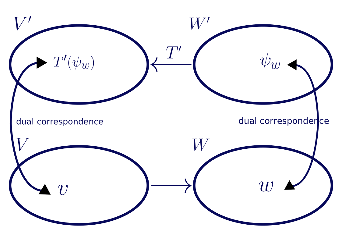
Recall the setup for Section 3F about a map that included the dual spaces, the dual map, and dual bases. In order to connect the dual map to the adjoint, we need to use the inner products on and If we have orthonormal bases for and then the correspondence between these spaces through their inner products will match the correspondence between the basis and dual basis. But recall that our bases were also built around the operator Here is a refresher.
is a basis for is an extension so that is a basis for Then is a basis for which can be extended to a basis for with the vectors We can make our original basis orthonormal by just applying Gram-Schmidt, which keep the first vectors as basis vectors for the kernel. So this would not change any of the arguments that followed. However, we didn't construct the basis of as the dual basis of this basis, so this doesn't help us immediately. We can also apply Gram-Schmidt to and this would mean that the inner product correspondence would take these new basis vectors to dual basis vectors. But we would no longer be able to know they were connected to the 's they originally came from. And there does not seem to be an immediate fix for this -- at least not in that section. Finally, there is not a clear connection between the dual basis vectors of we get from and the basis vectors for That's a very important road-block to being able to compute or understand the adjoint map through the dual map.
We will see in this section that 1) is an operator that has a basis of eigenvectors with non-negative eigenvalues, and
2) The square root of faithfully represents up to an isometry, i.e. there exists an isometry such that
Another way of thinking about this is that has an orthonormal basis with the property that is a basis for the kernel, and is an orthogonal basis for the range of (It would only be orthonormal if all of 's singular values are ) You can then find any orthonormal basis you like for because that is the kernel of and those dual vectors will have nothing to do with anything in the range of Furthermore, if we take dual bases of the orthonormal bases just described for and then sends each of the basis vectors back into the span of
Lemma: Properties of
Suppose Then a) is a positive operator on b) c) d)
Proof:
a) We first verify that is self-adjoint: To conclude, we let and show:
b) We will show the first inclusion, since the second is clear: If then
so c) This part follows from part (b) and the kernel/range relationship between adjoints:
d) The first equality follows from the setup in 3F, where the vectors were a basis for and the corresponding dual basis vectors in were a basis for Now, and have the same dimension, and in fact if we had constructed our setup for 3F with orthonormal bases and extension (in particular, if Gram-Schmidtt had been applied to the 's before extending to a basis for ) then they would have been corresponding vectors, i.e., would have also been a basis for The second equality follows directly from part (c).
Definition: Singular Values
Suppose The singular values of are nonnegative square roots the eigenvalues of , listed in decreasing order, each included as many times as the dimension of the corresponding eigenspace (i.e. geometric multiplicity).
Lemma: Role of Singular Values
Suppose Then a) is injective is not a singular value of b) The number of positive singular values of equals c) is surjective the number of positive singular values of is
Proof:
a) Since , we can conclude that is injective is injective is not an eigenvalue of b) Spectral theorem proves this: We have an orthogonal decomposition of eigenspaces and the kernel is just one of them (for ). If you remove the basis vectors that are in the kernel, you have a basis for the range, and that number is the same as the number of positive singular values (remember that we have one sigular value for each dimension for its corresponding eigenspace). c) This follows from part (b): We just established that the range has the same dimension as this number. Now, that's equal to the dimension of W if and only if is surjective.
Comparing Eigenvalues and Singular Values
Helpful Table from Axler's Linear Algebra Done Right
| Property | Eigenvalues | Singular Values |
|---|---|---|
| Applies to | Linear operators | Linear maps |
| Nature of values | Can be any scalar (may be complex, negative, or not exist over | Always real and non-negative (). Guaranteed to exist. |
| Associated vectors | Operates on a single non-zero vector such that . | Connects two orthonormal bases and such that . |
| Matrix representation | has a diagonal matrix with respect to some basis if and only if is diagonalizable. | always has a diagonal matrix with respect to some pair of orthonormal bases (Singular Value Theorem). |
| Relationship to adjoint | Eigenvalues of are the absolute squares of the eigenvalues of (only if is normal). | Singular values of are exactly the square roots of the eigenvalues of the positive operator . |
Corollary: Isometries characterized by having all singular values equal to
Suppose Then is an isometry all of the singular values of are
Proof:
We begin by noting that is an isometry if and only if is its inverse, i.e. Then the result follows, since the singular values are the diagonal entries of the diagonalized
SVD for Linear Maps and Matrices
Content
Lemma: Singular Value Decomposition
Suppose and the positive singular values of are Then there exist orthonormal lists in and in such that for every
Proof:
The orthonormal basis can be taken as orthonormal bases for each eigenspace (or just apply spectral theorem) for the operator The orthonormal basis is found by scaling each by This results in an orthonormal basis for because these images are all orthogonal and their norms are their corresponding singular value squared. Here is the verification of that fact:
Theorem: Singular Value Decomposition of Adjoint and Pseudoinverse
Suppose and the positive singular values of are Let , and be orthonormal lists in and respectively such that for every , Then a)
b)
Proof:
a) This is a formula for , so without effecting the outcome we can replace with projected onto , the orthogonal complement of Projecting this way makes this much easier to compute, since we have such a nice basis for Projected is , which is Then is the operator applied to Now, scales each basis vector by its respective , we have
b) Let us start by retracing the same steps that we took for the last proof. was first projected onto the range, This is the first step in computing the pseudoinverse. Then applying gives us the result However, this is not something in the pre-image of our projected It is the we are looking for after the application of But because just scales the th basis vector by , we can divide each element by to obtain what we want. This is not the only pre-image vector for , but it is the one with the smallest norm because adding anything in the kernel of , which is the orthogonal complement of the span of these basis vectors, would only increase the norm of the given vector. Therefore
Lemma: Matrix Version of SVD
Suppose is an -by- matrix of rank Then there exist an -by- matrix with orthonormal columns, an -by- diagonal matrix with positive numbers on the diagonal, and an -by- matrix with orthonormal columns such that
Proof:
Let us observe what does to a basis vector from the SVD of as an operator, verify that it is sent to , and then we will check that everything in the kernel of , which is the orthogonal complement of the span of these s, is sent to First, is sent by to the standard th basis vector. This is sent to the th column of , which is times the th standard basis vector by , and then sends this to , since is the th column of Now, the kernel of is the orthogonal complement of the span of the 's, so has columns all orthogonal to it and it is mapped to by